Procedure for creating a metabolic model for FBA

SysBioGTU

CONTRIBUTORS: Written: Regan ODONGO, Edited: Tunahan ÇAKIR

FBA Implementation Steps

Define the system’s boundary (e.g. cell wall).
Make ready the reaction list, which makes up the metabolic network. The reactions should be divided into two groups as follows:
- Internal reactions i.e. reactions confined within the system’s boundary. These should be written as well-balanced equations based on their reaction stoichiometries, with reactants on the left-hand side and products on the right-hand side.
- Exchange reactions i.e. reactions for metabolites taken up or released outside the system’s boundary
  
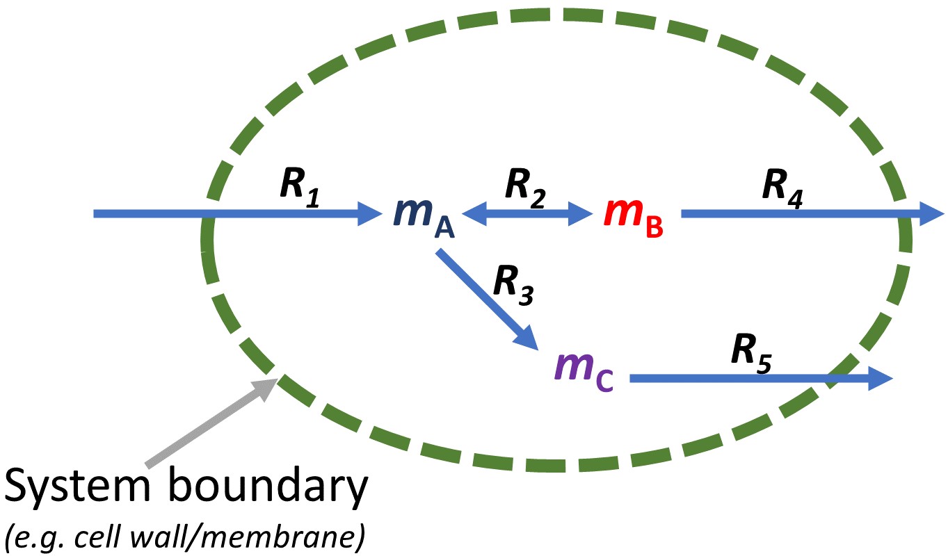
  From the figure above, for metabolites, mA, entering the system, the reaction is written as:
  
  $\to m_A$
  
  i.e. metabolite A is introduced into the system from outside the system’s boundary (an uptake reaction).
  
  On the other hand, for metabolites leaving the system, mB and mC, the reaction is written as:
  
  $\to m_B$
  
  $\to m_C$
  
  i.e. metabolite B and C are secreted out of the system.
  
  For the system defined in the figure above, the set of reactions in the system can be written as:
  
  $\begin{align} \to m_A \qquad... \qquad{R_1}\\ {m_A} {\leftrightarrow} {m_B} \qquad... \qquad{R_2}\\ {m_A} \leftrightarrow {m_C} \qquad... \qquad{R_3}\\ {m_B} \rightarrow \qquad... \qquad{R_4}\\ {m_C} \rightarrow \qquad... \qquad{R_5} \end{align}$
Write differential mass balances around intracellular metabolites.

For each intracellular metabolite, its amount within the system boundary (within the cell) will be increased by the reactions that produce it while the corresponding amount/pool will be consumed up by the reactions that use it as a substrate. That is, the intracellular metabolite concentrations over time will change as a function of the reaction rates that consume or produce them. This can be represented as a series of differential mass balances around intracellular metabolites as shown below:

$\begin{align} \frac{dm_A}{dt} &= R_1 - R_2 - R_3 \\ \frac{dm_B}{dt} &= R_2 - R_4\\ \frac{dm_C}{dt} &= R_3 - R_5 \end{align}$

The major assumption made by FBA is steady-state assumption. That is, there won’t be any net accumulation of intracellular metabolites over sufficiently long time. Under this assumption, the right-hand side of the equations above will be zero, leading to a system of linear equations to be solved for the prediction of metabolic fluxes (reaction rates).

$\begin{align} R_1 - R_2 - R_3 &= 0 \\ R_2 - R_4 &= 0\\ R_3 - R_5 &= 0 \end{align}$
Represent the set of equations derived from mass balances in matrix format.

The system of linear equations derived above can be represented in matrix format as given below. $\begin{align} S.v &= b \end{align}$

$\left\{ \begin{array}{c} {S_{11}}{v_1} + {S_{12}}{v_2} + ... {S_{1n}}{v_n} = 0 \\ {S_{21}}{v_1} + {S_{22}}{v_2} + ... {S_{2n}}{v_n} = 0 \\ ........... \\ {S_{m1}}{v_1} + {S_{m2}}{v_2} + ... {S_{mn}}{v_n} = 0 \end{array} \right.$

and for the example given previously,

$\begin{align} R_1 - R_2 - R_3 &= 0 \\ R_2 - R_4 &= 0\\ R_3 - R_5 &= 0 \end{align}$

The coefficients of unknowns in those equations indeed correspond to the stoichiometric coefficients of metabolites in the reaction list.
- Create a right-hand side zero vector (b). Its dimension must be m×1
$\begin{align} b &= \left( 0 \qquad0 \qquad0\right) \end{align}$

for each of the mass balance equations $\frac{dm_A}{dt}$ $\frac{dm_B}{dt}$ $\frac{dm_C}{dt}$
- Construct the stoichiometric matrix (e.g. in Excel). In this matrix, the rows represent the metabolites while the columns represent the reactions. For a system with m metabolites and n reactions, the resultant stoichiometric/coefficient matrix will have an m×n dimension. Care should be taken to ensure that the coefficient values are correctly defined to avoid errors in subsequent steps. For every reaction, the stoichiometric coefficient values of metabolites produced by the reaction are declared with positive values while those for metabolites consumed by the reaction are declared with negative values. All other metabolites are assigned with zero values for that reaction (column) in the stoichiometric matrix. Following is an example of a stoichiometric matrix derived from the system of linear equations defined in the previous step:
For convenience, such small networks, after defining in Excel worksheet, can be saved as a MATLAB object in a .mat file object format. An alternative is to use R, which we describe later. In MATLAB, this can be done as follows:
```
- Load the Excel file using stoichMat = xlsread(‘filename.xlsx’), assuming the file is named as ‘filename.xlsx’.

- Next, use save(‘stoichMat.mat’,’ stoichMat’,’mat’) to save the matrix as a .mat file object. Note that should the input file be large, other options in the ‘save’ function would be needed.

- This .mat file can be introduced into the working space memory of MATLAB using the ‘load’ function, e.g.load(‘stoichMat.mat’).
```
Define the other system constraints: Three main constraints are defined: mass-balance based stoichiometric constraints, reversibility constraints and measurement constraints:
- Stoichiometric constraint: already defined using the stoichiometric matrix as explained above. Care must be taken as numerical problems may be experienced should the stoichiometric matrix be wrongly defined.
- Reversibility constraints: Here, two vectors, lower-bound vector and upper-bound vector are constructed to define the lower and upper bounds of the rates of reactions in the system based on reaction irreversibility. If the system has n reactions, the dimensions of the resulting vectors will be n×1. Based on reaction irreversibility, for a reversible reaction, R~i, lb~i=-Infinity while the ub_i=+Infinity. On the other hand, if the reaction is an irreversible reaction, then, lb_i=0 while the ub_i=+Infinity. It is always better to use large values such as 1,000 in place of infinity.
- Measurement Constraints: If a measured physiological flux rate is available, the index of the corresponding reaction(s) in the ub and lb vectors should be defined using this value. For instance, if R_1is measured as 3 mmol/gram dry weight/hr, the ub and lb will be defined as follows:
  
  $\begin{array}{c|lcr} & {V_1} & {V_2} & {V_3}& {V_4}& {V_5} \\ \hline {m_A} & 1 & -1& -1 & 0 & 0 \\ {m_B} & 0 & 1& 0 & -1 & 0 \\ {m_C} & 0 & 0& 1 & 0 & -1 \end{array}$
Optimize the system based on the defined constraints. The example defined above is a typical linear system of equations that can be solved by most optimization programs. The MATLAB’s optimization toolbox has a base linprog function for handling such linear programming problems. This function, however, is less robust for the case of more complex models (e.g. those with over 30 reactions). Instead, GLPK solver can be used for such models. This is a free linear programming solver with a MATLAB interface. To install it in MATLAB, download the latest version form this link: http://sourceforge.net/projects/glpkmex/files/glpkmex/2.11/. Unzip the file into a folder and add the folder to the MATLAB’s current path by following File -> SetPath in the MATLAB menu bar and browsing to find right folder. A rather much stable solver is Gurobi that can be found here: https://www.gurobi.com/downloads/gurobi-optimizer-eula/. A free 3-month academic license can be obtained by signing up using your institutional (university given) e-mail address in this link: https://www.gurobi.com/academia/academic-program-and-licenses/. As compared to other solvers, Gurobi is much easier to use as shown below.

Please see how this can be done in MATLAB and R