A Small Scale Metabolic Model of Corynebacterium glutamicum

CONTRIBUTORS

MATLAB file: Ecehan Abdik, R file: Elif Emanetci, Excel file: İsa Yüksel, MATLAB Live Editor: Kadir Kocabaş, R Markdown: H. Büşra Lüleci, Editing: Tunahan Çakır

1. About the Model

Corynebacterium glutamicum is a bacterium used for industrial production of amino acids. It was initially discovered as a glutamate producer, as the name suggests. Vallino et al. (1993) constructed a small-scale metabolic network to determine basal metabolic flux distribution of C.glutamicum for lysine overproduction using stoichiometric mass balancing [1]. Their metabolic network consists of 34 intracellular metabolic reactions and 37 metabolites. 12 of those metabolites are exchanged with the extracellular environment. The authors collected experimental data to validate the metabolic network by growing the organism in batch fermentation. They broke down the batch fermentation into four separate phases and calculated metabolic fluxes for each phase separately (see Figure 2A of the paper [1]). The mass balance equations were constructed around the 37 intracellular metabolites. They used measured uptake/release rates of 12 extracellular metabolites to calculate metabolic flux distributions by a least-square approach since their system was overdetermined. The extracellular metabolites are glucose, oxygen, ammonium, CO2, biomass, acetate, alanine, lactate, lysine, pyruvate, trehalose and valine. We rearranged their metabolic network as COBRA compatible .mat file and sbml file, both of which can be used to apply Flux Balance Analysis (FBA). The model is also available in stoichiometric matrix format and in reaction list format in an Excel file. The rearranged metabolic network accessible via those files has 34 intracellular metabolic reactions and 14 exchange reactions. Below, we run the model for phase I of the batch fermentation. The metabolic fluxes predicted by the authors for this phase are given in Figure 4 of their paper [1]. The model has 48 unknowns (number of reactions) and 42 independent equations (rank of the stoichiometric matrix). Therefore, the degrees of freedom (dof) of the model is 6. In oppose to the overdetermined solution strategy in the original paper, here we aimed to solve the system using FBA, which requires an underdetermined system (dof > 0). We wanted to predict values as close as possible to Figure 4 of the paper at the same time. Therefore, we used five measured flux rates (exchange reactions of ammonium, glucose, lactate, oxygen and trehalose) as constraints in the simulations below, making dof value 1.

2. Reading or Loading the model

We provide two alternatives to import the metabolic model to MATLAB. The first one (denoted as case 1 below) is reading the model from the sbml file by using readCbModel of COBRA Toolbox. The second one (denoted as case 2 below) is loading the provided .mat file to MATLAB. prefer=input(['Would you prefer to read sbml formatted model or load mat formatted model? ' ... '(enter 1 for reading or 2 for load): ']);

    switch prefer
        case 1
            model=readCbModel('Vallino_COBRAtc.xml');
        case 2
            load('Vallino.mat')
    end

3. Exploring metabolic model

There are three main fields in the metabolic models.

a) Stoichiometric Matrix (S Matrix) = It is a two dimensional numeric matrix that represents coefficients in metabolic reactions. Columns and rows represent reactions (unknowns) and metabolites (equations) respectively (See FBA Primer page for details).

b) mets = It is the list of metabolites included in the model reactions. Here, metabolites are usually represented by abbreviations. To display the first 5 metabolites in the model (i.e.the metabolites corresponding to the first 5 rows of S matrix): model.mets(1:5)

c) rxns = It is the list of all reactions in the model. The names/IDs of reactions are stored here. To display the first 5 reactions in the model (i.e.the reactions corresponding to the first 5 columns of S matrix): model.rxns(1:5)

4. Formatting for Gurobi optimization solver

There are a couple of optimization solvers that can be used to predict the flux distributions for underdetermined metabolic models. The most common ones are glpk, Gurobi and IBM CPLEX. Among those, glpk is a free solver, and free academic license is available for Gurobi and CPLEX. Gurobi requires a specific model structure that can be created by using the information in the .mat formatted or .sbml derived metabolic model. Structure of Gurobi model: A = The stoichiometric matrix, which holds all the equations in matrix format, must be named as A. The matrix is conventionally named as S in metabolic modeling literature. lb = The lower bound vector of the reactions (minimum allowable rates for reactions) must be named as lb. ub = The upper bound vector of the reactions (maximum allowable rates for reactions) must be named as ub. rhs = The right hand side vector in the mass-balance-based FBA equation (S.v = b) must be named as rhs. It is conventionally named as b in metabolic modeling literature (Figure 2). obj= The vector that defines objective function coefficients must be named as obj. Negative coefficient indicates maximization while positive coefficient indicates minimization. It is conventionally named as f in metabolic modeling literature. sense= The cell array that shows whether an equation defines equality or inequality. Since all mass-balance based equations in FBA are equality equations, all elements of sense array must be "=". vtype= The cell array that defines whether an unknown is continuous, binary or integer. Since our unknowns (reaction rates) are continuous, all elements of vtype array must be "C".

    Gurobimodel.A  = [model.S]; % Stochiomatrix format for gurobi showen as A instead of S
    Gurobimodel.A  = sparse(Gurobimodel.A); % Gurobi requires A as a sparse matrix
    Gurobimodel.lb = model.lb;
    Gurobimodel.ub = model.ub;
    Gurobimodel.rhs= zeros(length(Gurobimodel.A(:,1)),1); 
    Gurobimodel.obj= zeros(length(Gurobimodel.A(1,:)),1); % objective function
    Gurobimodel.sense = ['=']; 
    Gurobimodel.vtype = 'C' ;

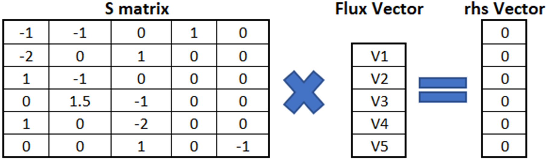
Figure 2 : S matrix

5. Defining Constraints for the Experimental Condition

Phase I of the batch fermentation will be simulated here. The experimentally measured secretion rates were taken from [2]. Although 12 exchange rates were measured by the authors, we use 5 of them here, which corresponds to an underdetermined system with degrees of freedom 1. The rates of corresponding exchange reactions are fixed to the experimental values by setting their upper and lower bounds to the same value. Gurobimodel.lb(35) = 100; Gurobimodel.ub(35)=100; % glucose uptake Gurobimodel.lb(36) = 68.3; Gurobimodel.ub(36)=68.3; % NH3 uptake Gurobimodel.lb(37) = 231; Gurobimodel.ub(37)=231; % O2 uptake Gurobimodel.lb(42) = 2.5; Gurobimodel.ub(42)= 2.5;% trehalose release Gurobimodel.lb(43) = 0.3; Gurobimodel.ub(43)= 0.3; % lactate release

6. Defining the Objective Function: Maximization of Growth

The biomass reaction is 33th reaction in the model. To maximize growth, 33th index of obj vector will be defined as -1, with all other indices set to zero. The obj vector was already initialized above (Section 4) as a zero vector. Gurobimodel.obj(33) = -1;

7. Running the Optimization and Exploring the Results

All necessary rearrangements were made in the previous steps (eg. defining the constraints and the objective function). Now, the function "gurobi" will be used to predict a flux distribution that corresponds to maximum growth rate for the defined constraints. phaseI = gurobi(Gurobimodel); Gurobi generates an output in structure format, with a couple of outputs. The most relevant outputs are objval and x. objval = reports the optimum value of the objective function. In this case, it will print the maximum growth rate for the defined constraints. To display the objective value: phaseI.objval x = reports the predicted flux vector. To display reaction rates (fluxes) of the first 5 reactions: phaseI.x(1:5)

8. Flux Variability Analysis (FVA)

The constraint-based modelling approach is a combination of mathematical techniques that optimize hundreds of mass balance derived equations written based on reactions inside organism of interest. In constraint-based metabolic models, alternate optima can be an issue in interpreting the results of FBA since there might be multiple flux distributions that result in the same value for the objective function (Figure 3). FVA method determines the maximum and minimum flux value of all reactions can take for the same objective value. In this section, firstly, upper and lower bound of the biomass reaction is set to the previously found maximum biomass production rate (in the Maximization of biomass section). Secondly, the maximum and minimum flux values of all reactions can take are determined by changing the objective function inside for loop. Gurobimodel.lb(33)=phaseI.x(33); Gurobimodel.ub(33)=phaseI.x(33); for i=1:length(Gurobimodel.A(1,:)) Gurobimodel.obj=zeros(length(Gurobimodel.A(1,:)),1); Gurobimodel.obj(i)=1; Vmin=gurobi(Gurobimodel,params); Gurobimodel.obj(i)=-1; Vmax=gurobi(Gurobimodel); FVA_I(i,:)=([Vmin.x(i) Vmax.x(i)]); end

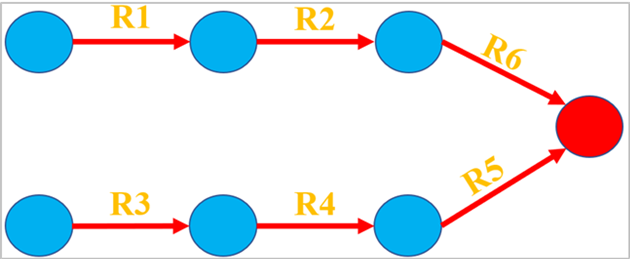
Figure 3: Representation of flux variability on a toy model. The red lines with arrow and R1,R2,R3,R4,R5 and R6 indicate irreversible reactions and reaction names respectively. The circles represent metabolites. Flux variability will be an issue if maximization of the red metabolite were chosen as objective function since it can be produced through R1, R2 and R6 as well as R3, R4 and R5 reaction chains.

IMPORTANT NOTE: You can access a MATLAB LiveScipt file of this tutorial from GitHub by following this link

References

• Vallino, J. J., & Stephanopoulos, G. (1993). Metabolic flux distributions in Corynebacterium glutamicum during growth and lysine overproduction. Biotechnology and Bioengineering, 41(6), 633-646.